Capítulo 7 Spatial modeling leukemia
7.1 Mortality
Spatial modeling of incidence and mortality childhood leukemia based on Colombian armed conflict and poverty for children born during the years 2002-2013
7.1.1 Packages Mortality
rm(list=ls())
require(rgdal)
require(pscl)
require(sf)
require(spdep)
require(spatialreg) #test.W, scores.listw
require(stringr)
require(performance)
require(AER)
require(ggplot2)
require(vcdExtra)
require(dbscan)
7.1.2 Code Mortality
- Reading the shapefile of 1124 Colombian municipalities, defining the Coordinate Reference System and centroid and building some variables
#Reading the shapefile of 1124 Colombian municipalities
muncol <- rgdal::readOGR(dsn="data_2_Leukemia/muncol.shp")
## Warning: OGR support is provided by the sf and terra packages among others## Warning: OGR support is provided by the sf and terra packages among others## Warning: OGR support is provided by the sf and terra packages among others## Warning: OGR support is provided by the sf and terra packages among others## Warning: OGR support is provided by the sf and terra packages among others## Warning: OGR support is provided by the sf and terra packages among others## Warning: OGR support is provided by the sf and terra packages among others## OGR data source with driver: ESRI Shapefile
## Source: "/home/jncc/Documents/Monitorias/EspacialPage/Clases-EE-UN/data_2_Leukemia/muncol.shp", layer: "muncol"
## with 1124 features
## It has 17 fieldsmuncol=spTransform(muncol,CRS("+init=epsg:21897"))## Warning: PROJ support is provided by the sf and terra packages among others(l <- length(muncol))## [1] 1124#Representative coordinate (centroid)
options(warn = -1)
xy0=data.frame(x=muncol$x,y=muncol$y)
coordinates(xy0) <- c('x','y')
proj4string(xy0) <- CRS("+init=epsg:4326")
xy0=spTransform(xy0,CRS("+init=epsg:21897"))
###Loops for avoiding NA
r <- sum(muncol$Ndeaths)/sum(muncol$NPop)
for (i in 1:l){
if(muncol$NPop[i]==0){
muncol$EsperadosDeNCancer[i] <- 1
}
else{
muncol$EsperadosDeNCancer[i] <- muncol$NPop[i]*r
}
}
muncol$IICA_Cat=muncol$IICA_Ca
muncol$IICA_Cat=str_replace_all(muncol$IICA_Cat,"Bajo", "Low")
muncol$IICA_Cat=str_replace_all(muncol$IICA_Cat,"Medio", "Medium")
muncol$IICA_CatLow=ifelse(muncol$IICA_Cat=="Low",1,0)
muncol$IICA_CatMed=ifelse(muncol$IICA_Cat=="Medium",1,0)
muncol$IICA_High=as.character(1-(muncol$IICA_CatLow+muncol$IICA_CatMed))
muncol$UBN=muncol$NBI- Modeling leukemia Mortality Rate (LR) in terms of Colombian armed conflict index, poverty, rurality and health coverage. First, the usual Poisson regression model with mortality rate as response variable is estimated.
glmbaseLMR<-glm(Ndeaths ~IICA_High+UBN+Per_Rur+Cobertura+offset(log(EsperadosDeNCancer)), family = poisson,data = muncol)
anova(glmbaseLMR)
## Analysis of Deviance Table
##
## Model: poisson, link: log
##
## Response: Ndeaths
##
## Terms added sequentially (first to last)
##
##
## Df Deviance Resid. Df Resid. Dev
## NULL 1123 799.92
## IICA_High 1 0.694 1122 799.22
## UBN 1 43.405 1121 755.82
## Per_Rur 1 4.017 1120 751.80
## Cobertura 1 9.185 1119 742.62muncol$residLMR=residuals(glmbaseLMR)
summary(glmbaseLMR)##
## Call:
## glm(formula = Ndeaths ~ IICA_High + UBN + Per_Rur + Cobertura +
## offset(log(EsperadosDeNCancer)), family = poisson, data = muncol)
##
## Deviance Residuals:
## Min 1Q Median 3Q Max
## -2.9317 -0.5949 -0.4108 -0.2389 3.3300
##
## Coefficients:
## Estimate Std. Error z value Pr(>|z|)
## (Intercept) -0.583783 0.307508 -1.898 0.05764 .
## IICA_High1 0.107822 0.084777 1.272 0.20343
## UBN -0.007902 0.003003 -2.632 0.00850 **
## Per_Rur -0.002705 0.002370 -1.141 0.25380
## Cobertura 0.991687 0.336039 2.951 0.00317 **
## ---
## Signif. codes: 0 '***' 0.001 '**' 0.01 '*' 0.05 '.' 0.1 ' ' 1
##
## (Dispersion parameter for poisson family taken to be 1)
##
## Null deviance: 799.92 on 1123 degrees of freedom
## Residual deviance: 742.62 on 1119 degrees of freedom
## AIC: 1271.7
##
## Number of Fisher Scoring iterations: 6Rurality and conflict armed index are not statistically significant in this first auxiliar model. However, we maintain these variables in the rest of the analysis and review its significance in the final model.
Checking excess zeros by comparison between the number of zeros predicted by the model with the observed number of zeros. Also checking overdispersion.
mu_LMR <- predict(glmbaseLMR, type = "response")  # predict expected mean count
expLMR <- sum(dpois(x = 0, lambda = mu_LMR))      # sum the probabilities of a zero count for each mean
round(expLMR)                                    #predicted number of zeros
## [1] 898sum(muncol$Ndeaths < 1) #observed number of zeros## [1] 907zero.test(muncol$Ndeaths) #score test (van den Broek, 1995)## Score test for zero inflation
##
## Chi-square = 902.95398
## df = 1
## pvalue: < 0.000000000000000222##Checking overdispersion
dispersiontest(glmbaseLMR) #Cameron & Trivedi (1990)##
## Overdispersion test
##
## data: glmbaseLMR
## z = 2.2049, p-value = 0.01373
## alternative hypothesis: true dispersion is greater than 1
## sample estimates:
## dispersion
## 1.109361The observed frequency of zeroes in data exceeds the predicted in the Leukemia mortality rate (LMR) model. Also, overdispersion is detected.
Now, to validate the independence assumption, first, it is necessary to define spatial weighting possible matrices.
rook_nb_b=nb2listw(poly2nb(muncol,queen=FALSE), style="B",zero.policy = TRUE)
rook_nb_w=nb2listw(poly2nb(muncol,queen=FALSE), style="W",zero.policy = TRUE)

queen_nb_b=nb2listw(poly2nb(muncol,queen=TRUE), style="B",zero.policy = TRUE)
queen_nb_w=nb2listw(poly2nb(muncol,queen=TRUE), style="W",zero.policy = TRUE)

#Graphs neighbours
trinb=tri2nb(xy0)
options(warn = -1)
tri_nb_b=nb2listw(tri2nb(xy0), style="B",zero.policy = TRUE)
tri_nb_w=nb2listw(tri2nb(xy0), style="W",zero.policy = TRUE)

soi_nb_b=nb2listw(graph2nb(soi.graph(trinb,xy0)), style="B",zero.policy = TRUE)
soi_nb_w=nb2listw(graph2nb(soi.graph(trinb,xy0)), style="W",zero.policy = TRUE)

relative_nb_b=nb2listw(graph2nb(relativeneigh(xy0), sym=TRUE), style="B",zero.policy = TRUE)
relative_nb_w=nb2listw(graph2nb(relativeneigh(xy0), sym=TRUE), style="W",zero.policy = TRUE)

gabriel_nb_b=nb2listw(graph2nb(gabrielneigh(xy0), sym=TRUE), style="B",zero.policy = TRUE)
gabriel_nb_w=nb2listw(graph2nb(gabrielneigh(xy0), sym=TRUE), style="W",zero.policy = TRUE)

#Distance neighbours

knn1_nb_b=nb2listw(knn2nb(knearneigh(xy0, k = 1)), style="B",zero.policy = TRUE)
knn1_nb_w=nb2listw(knn2nb(knearneigh(xy0, k = 1)), style="W",zero.policy = TRUE)
knn2_nb_b=nb2listw(knn2nb(knearneigh(xy0, k = 2)), style="B",zero.policy = TRUE)
knn2_nb_w=nb2listw(knn2nb(knearneigh(xy0, k = 2)), style="W",zero.policy = TRUE)
knn3_nb_b=nb2listw(knn2nb(knearneigh(xy0, k = 3)), style="B",zero.policy = TRUE)
knn3_nb_w=nb2listw(knn2nb(knearneigh(xy0, k = 3)), style="W",zero.policy = TRUE)
knn4_nb_b=nb2listw(knn2nb(knearneigh(xy0, k = 4)), style="B",zero.policy = TRUE)
knn4_nb_w=nb2listw(knn2nb(knearneigh(xy0, k = 4)), style="W",zero.policy = TRUE)

mat=list(rook_nb_b,rook_nb_w,
         queen_nb_b,queen_nb_w,
         tri_nb_b,tri_nb_w,
         soi_nb_b,soi_nb_w,
         gabriel_nb_b,gabriel_nb_w,
         relative_nb_b,relative_nb_w,
         knn1_nb_b,knn1_nb_w,
         knn2_nb_b,knn2_nb_w,
         knn3_nb_b,knn3_nb_w,
knn4_nb_b,knn4_nb_w)- Testing spatial autocorrelation using Moran index test based on weighting matrices built in the last step. Note that with all weighting matrices we obtain a significant spatial autocorrelation.
aux=numeric(0)
options(warn = -1)
{
for(i in 1:length(mat))
aux[i]=moran.test(muncol$residLMR,mat[[i]],alternative="two.sided")$"statistic"
aux
}
## [1] 1.238996 1.473832 1.428553 1.629968 1.367192 1.592464 1.921616 2.011106 1.860100 2.247294 2.629440
## [12] 2.588622 1.099401 1.099401 2.469062 2.469062 3.088200 3.088200 3.450986 3.450986which.max(aux)## [1] 19moran.test(muncol$residLMR, mat[[which.max(aux)]], alternative="two.sided")##
## Moran I test under randomisation
##
## data: muncol$residLMR
## weights: mat[[which.max(aux)]]
##
## Moran I statistic standard deviate = 3.451, p-value = 0.0005585
## alternative hypothesis: two.sided
## sample estimates:
## Moran I statistic Expectation Variance
## 0.0672352967 -0.0008904720 0.0003897053- First, Poisson Hurdle model is estimated without consider spatial autocorrelation.
mod.hurdleLMR <- hurdle(Ndeaths ~IICA_High+UBN+Per_Rur+Cobertura+offset(log(EsperadosDeNCancer))|IICA_High+UBN+Per_Rur+Cobertura+offset(log(EsperadosDeNCancer)),data = muncol,dist = "poisson", zero.dist = "binomial")
resid_Pois_Hurdle=residuals(mod.hurdleLMR,"response")
summary(mod.hurdleLMR)
##
## Call:
## hurdle(formula = Ndeaths ~ IICA_High + UBN + Per_Rur + Cobertura + offset(log(EsperadosDeNCancer)) |
## IICA_High + UBN + Per_Rur + Cobertura + offset(log(EsperadosDeNCancer)), data = muncol, dist = "poisson",
## zero.dist = "binomial")
##
## Pearson residuals:
## Min 1Q Median 3Q Max
## -1.6105 -0.4155 -0.2926 -0.1781 7.8519
##
## Count model coefficients (truncated poisson with log link):
## Estimate Std. Error z value Pr(>|z|)
## (Intercept) 0.0131708 0.3793725 0.035 0.9723
## IICA_High1 0.2239159 0.1048208 2.136 0.0327 *
## UBN -0.0006294 0.0050823 -0.124 0.9014
## Per_Rur -0.0064173 0.0049162 -1.305 0.1918
## Cobertura 0.1702217 0.4227398 0.403 0.6872
## Zero hurdle model coefficients (binomial with logit link):
## Estimate Std. Error z value Pr(>|z|)
## (Intercept) -1.013658 0.570592 -1.777 0.075650 .
## IICA_High1 -0.091317 0.177363 -0.515 0.606652
## UBN -0.011792 0.004690 -2.514 0.011928 *
## Per_Rur -0.005190 0.003982 -1.303 0.192473
## Cobertura 2.283308 0.624231 3.658 0.000254 ***
## ---
## Signif. codes: 0 '***' 0.001 '**' 0.01 '*' 0.05 '.' 0.1 ' ' 1
##
## Number of iterations in BFGS optimization: 10
## Log-likelihood: -624 on 10 DfpR2(mod.hurdleLMR)## fitting null model for pseudo-r2## llh llhNull G2 McFadden r2ML r2CU
## -623.9804020 -1369.2239672 1490.4871304 0.5442817 0.7344776 0.8048896moran.test(resid_Pois_Hurdle, mat[[which.max(aux)]], alternative="two.sided")##
## Moran I test under randomisation
##
## data: resid_Pois_Hurdle
## weights: mat[[which.max(aux)]]
##
## Moran I statistic standard deviate = 4.8924, p-value = 0.0000009964
## alternative hypothesis: two.sided
## sample estimates:
## Moran I statistic Expectation Variance
## 0.0935041339 -0.0008904720 0.0003722701- Only Conflict armed index predictor is significant but model residuals are significantly spatially autocorrelated. So, we use spatial filtering and check significance again. Below we find Moran Eigenvectors.
MEpoisLMR <- spatialreg::ME(Ndeaths ~ IICA_High+UBN+Per_Rur+Cobertura+offset(log(EsperadosDeNCancer)),data=muncol,family="poisson",listw=knn4_nb_b, alpha=0.02, verbose=TRUE)## eV[,11], I: 0.02918226 ZI: NA, pr(ZI): 0.04MoranEigenVLMR=data.frame(fitted(MEpoisLMR))
#summary(MoranEigenVLMR)- Now, we used Poisson Hurdle model to manage the overdispersion due to zero excess and Moran eigenfunctions are included as additional explanatory variables, so that spatial autocorrelation is considered.
mod.hurdleLMR <- hurdle(
  Ndeaths ~ IICA_High+UBN+Per_Rur+Cobertura+
            fitted(MEpoisLMR)+offset(log(EsperadosDeNCancer))|IICA_High+
            UBN+Per_Rur+Cobertura+offset(log(EsperadosDeNCancer)),
  data = muncol,
  dist = "poisson",
  zero.dist = "binomial")

resid_Pois_Hurdle=residuals(mod.hurdleLMR,"response")
summary(mod.hurdleLMR)
##
## Call:
## hurdle(formula = Ndeaths ~ IICA_High + UBN + Per_Rur + Cobertura + fitted(MEpoisLMR) + offset(log(EsperadosDeNCancer)) |
## IICA_High + UBN + Per_Rur + Cobertura + offset(log(EsperadosDeNCancer)), data = muncol, dist = "poisson",
## zero.dist = "binomial")
##
## Pearson residuals:
## Min 1Q Median 3Q Max
## -1.6969 -0.4153 -0.2920 -0.1791 7.8744
##
## Count model coefficients (truncated poisson with log link):
## Estimate Std. Error z value Pr(>|z|)
## (Intercept) 0.374295 0.391853 0.955 0.33948
## IICA_High1 0.286868 0.104433 2.747 0.00602 **
## UBN -0.010727 0.005917 -1.813 0.06986 .
## Per_Rur -0.003464 0.005096 -0.680 0.49664
## Cobertura -0.058726 0.436141 -0.135 0.89289
## fitted(MEpoisLMR) -8.856022 1.670191 -5.302 0.000000114 ***
## Zero hurdle model coefficients (binomial with logit link):
## Estimate Std. Error z value Pr(>|z|)
## (Intercept) -1.013658 0.570592 -1.777 0.075650 .
## IICA_High1 -0.091317 0.177363 -0.515 0.606652
## UBN -0.011792 0.004690 -2.514 0.011928 *
## Per_Rur -0.005190 0.003982 -1.303 0.192473
## Cobertura 2.283308 0.624231 3.658 0.000254 ***
## ---
## Signif. codes: 0 '***' 0.001 '**' 0.01 '*' 0.05 '.' 0.1 ' ' 1
##
## Number of iterations in BFGS optimization: 12
## Log-likelihood: -610 on 11 DfpR2(mod.hurdleLMR)## fitting null model for pseudo-r2## llh llhNull G2 McFadden r2ML r2CU
## -610.0288758 -1369.2239672 1518.3901828 0.5544711 0.7409880 0.8120241moran.test(resid_Pois_Hurdle, mat[[which.max(aux)]], alternative="two.sided")##
## Moran I test under randomisation
##
## data: resid_Pois_Hurdle
## weights: mat[[which.max(aux)]]
##
## Moran I statistic standard deviate = 1.4546, p-value = 0.1458
## alternative hypothesis: two.sided
## sample estimates:
## Moran I statistic Expectation Variance
## 0.027522708 -0.000890472 0.000381564- Rurality and health coverage are not statistically significant for counto model. So, those predictors are excluded of the spatial filtering and model.
MEpoisLMR <- spatialreg::ME(
  Ndeaths ~ IICA_High+UBN+offset(log(EsperadosDeNCancer)),
  data=muncol,
  family="poisson",
  listw=knn4_nb_b,
  alpha=0.02,
  verbose=TRUE)
## eV[,11], I: 0.01071212 ZI: NA, pr(ZI): 0.17MoranEigenVLMR=data.frame(fitted(MEpoisLMR))
#summary(MoranEigenVLMR)mod.hurdleLMR <- hurdle(
Ndeaths ~ IICA_High+UBN+fitted(MEpoisLMR)+
offset(log(EsperadosDeNCancer))|UBN+Cobertura+offset(log(EsperadosDeNCancer)),
data = muncol,
dist = "poisson",
zero.dist = "binomial")
summary(mod.hurdleLMR)##
## Call:
## hurdle(formula = Ndeaths ~ IICA_High + UBN + fitted(MEpoisLMR) + offset(log(EsperadosDeNCancer)) |
## UBN + Cobertura + offset(log(EsperadosDeNCancer)), data = muncol, dist = "poisson", zero.dist = "binomial")
##
## Pearson residuals:
## Min 1Q Median 3Q Max
## -1.5905 -0.4184 -0.2973 -0.1823 7.3265
##
## Count model coefficients (truncated poisson with log link):
## Estimate Std. Error z value Pr(>|z|)
## (Intercept) 0.355460 0.097724 3.637 0.000275 ***
## IICA_High1 0.274468 0.100011 2.744 0.006062 **
## UBN -0.013803 0.003796 -3.636 0.000277 ***
## fitted(MEpoisLMR) -9.134355 1.617421 -5.647 0.0000000163 ***
## Zero hurdle model coefficients (binomial with logit link):
## Estimate Std. Error z value Pr(>|z|)
## (Intercept) -1.279352 0.535993 -2.387 0.016992 *
## UBN -0.014391 0.004288 -3.356 0.000789 ***
## Cobertura 2.354642 0.616661 3.818 0.000134 ***
## ---
## Signif. codes: 0 '***' 0.001 '**' 0.01 '*' 0.05 '.' 0.1 ' ' 1
##
## Number of iterations in BFGS optimization: 11
## Log-likelihood: -611.3 on 7 DfpR2(mod.hurdleLMR)## fitting null model for pseudo-r2## llh llhNull G2 McFadden r2ML r2CU
## -611.2637930 -1369.2239672 1515.9203483 0.5535692 0.7404182 0.8113997moran.test(resid_Pois_Hurdle, mat[[which.max(aux)]], alternative="two.sided")##
## Moran I test under randomisation
##
## data: resid_Pois_Hurdle
## weights: mat[[which.max(aux)]]
##
## Moran I statistic standard deviate = 1.4546, p-value = 0.1458
## alternative hypothesis: two.sided
## sample estimates:
## Moran I statistic Expectation Variance
## 0.027522708 -0.000890472 0.000381564- Now, Poisson-Hurdle model residuals are not significant spatially autocorrelated. The LMR’s positive values depend only on the Index of armed conflict (IICA) and on the unsatisfied basic needs index (UBN) and LMR’s zero values depend on the UBN and health coverage. Note that the model shows good performance, according to pseudo R2 and the comparison between observed and predicted frequencies.
mf <- model.frame(mod.hurdleLMR)
y <- model.response(mf)
w <- model.weights(mf)
if(is.null(w)) w <- rep(1, NROW(y))
max0 <- 20L
obs <- as.vector(xtabs(w ~ factor(y, levels = 0L:max0)))
exp <- colSums(predict(mod.hurdleLMR, type = "prob", at = 0L:max0) * w)

fitted_vs_observed <- data.frame(Expected = exp,
                                 Observed = obs)
data <- reshape2::melt(fitted_vs_observed)
## No id variables; using all as measure variablesdata <- data.frame(data, x = 0:20)
data1 <- data[1:21, ]
data2 <- data[22:42, ]
pMortality <- ggplot() +
geom_line(data1, mapping = aes(x = x, y = value, group = variable
, color = variable)) +
geom_point(data1, mapping = aes(x = x, y = value, group = variable,
color = variable)) +
geom_col(data2, mapping = aes(x = x, y = value, group = variable),
alpha = 0.7) +
theme_light() +
labs(x = "Number of deaths",
y = "Frecuencies")
pMortality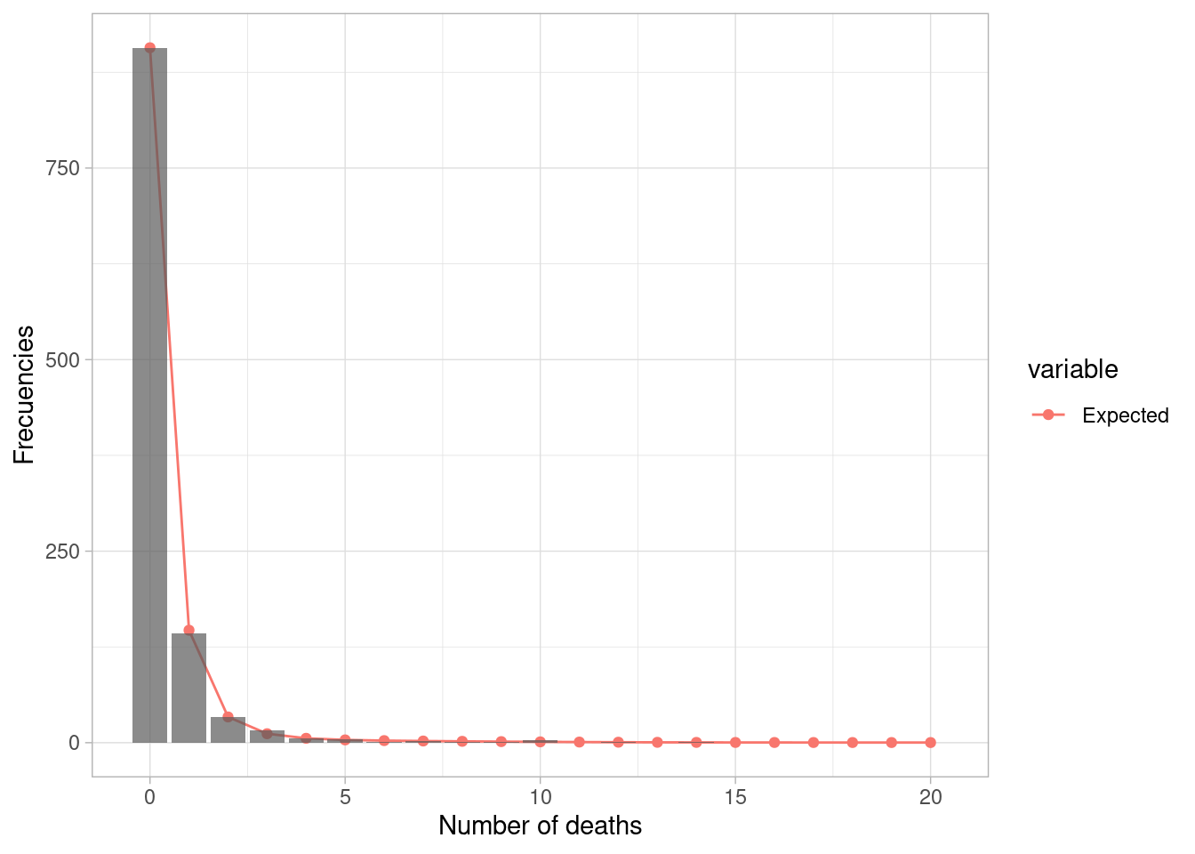
7.2 Incidence
Spatial modeling of incidence and mortality childhood leukemia based on Colombian armed conflict and poverty for children born during the years 2002-2013
7.2.1 Packages Incidence
rm(list=ls())
require(rgdal)
require(pscl)
require(sf)
require(spdep)
require(spatialreg) #test.W, scores.listw
require(stringr)
require(performance)
require(AER)
require(ggplot2)
require(vcdExtra)
7.2.2 Code Incidence
- Reading the shapefile of 1124 Colombian municipalities, defining the Coordinate Reference System and centroid and building some variables
#Reading the shapefile of 1124 Colombian municipalities
muncol <- rgdal::readOGR(dsn="data_2_Leukemia/muncol.shp")
## OGR data source with driver: ESRI Shapefile
## Source: "/home/jncc/Documents/Monitorias/EspacialPage/Clases-EE-UN/data_2_Leukemia/muncol.shp", layer: "muncol"
## with 1124 features
## It has 17 fieldsmuncol=spTransform(muncol,CRS("+init=epsg:21897"))
(l <- length(muncol))## [1] 1124#Representative coordinate (centroid)
xy0=data.frame(x=muncol$x,y=muncol$y)
coordinates(xy0) <- c('x','y')
proj4string(xy0) <- CRS("+init=epsg:4326")
xy0=spTransform(xy0,CRS("+init=epsg:21897"))
###Loops for avoiding NA
r <- sum(muncol$NCases)/sum(muncol$NPop)
for (i in 1:l){
if(muncol$NPop[i]==0){
muncol$EsperadosNCancer[i] <- 1
}
else{
muncol$EsperadosNCancer[i] <- muncol$NPop[i]*r
}
}
muncol$IICA_Cat=muncol$IICA_Ca
muncol$IICA_Cat=str_replace_all(muncol$IICA_Cat,"Bajo", "Low")
muncol$IICA_Cat=str_replace_all(muncol$IICA_Cat,"Medio", "Medium")
muncol$IICA_CatLow=ifelse(muncol$IICA_Cat=="Low",1,0)
muncol$IICA_CatMed=ifelse(muncol$IICA_Cat=="Medium",1,0)
muncol$IICA_High=as.character(1-(muncol$IICA_CatLow+muncol$IICA_CatMed))
muncol$UBN=muncol$NBI- Modeling leukemia Incidence Rate (LR) in terms of Colombian armed conflict index, poverty and rurality. First, the usual Poisson regression model with incidence rate as response variable is estimated.
glmbaseLR<-glm(
  NCases ~ IICA_High+UBN+Per_Rur+
          offset(log(EsperadosNCancer)),
  family = poisson,data = muncol)

anova(glmbaseLR)
## Analysis of Deviance Table
##
## Model: poisson, link: log
##
## Response: NCases
##
## Terms added sequentially (first to last)
##
##
## Df Deviance Resid. Df Resid. Dev
## NULL 1123 2524.9
## IICA_High 1 0.75 1122 2524.1
## UBN 1 328.90 1121 2195.2
## Per_Rur 1 0.11 1120 2195.1summary(glmbaseLR)##
## Call:
## glm(formula = NCases ~ IICA_High + UBN + Per_Rur + offset(log(EsperadosNCancer)),
## family = poisson, data = muncol)
##
## Deviance Residuals:
## Min 1Q Median 3Q Max
## -5.1779 -1.1632 -0.5270 0.6082 7.7193
##
## Coefficients:
## Estimate Std. Error z value Pr(>|z|)
## (Intercept) 0.3226036 0.0276280 11.677 < 0.0000000000000002 ***
## IICA_High1 0.0818208 0.0294297 2.780 0.00543 **
## UBN -0.0123797 0.0010425 -11.875 < 0.0000000000000002 ***
## Per_Rur -0.0002510 0.0007692 -0.326 0.74419
## ---
## Signif. codes: 0 '***' 0.001 '**' 0.01 '*' 0.05 '.' 0.1 ' ' 1
##
## (Dispersion parameter for poisson family taken to be 1)
##
## Null deviance: 2524.9 on 1123 degrees of freedom
## Residual deviance: 2195.1 on 1120 degrees of freedom
## AIC: 4174.2
##
## Number of Fisher Scoring iterations: 5muncol$residLR=residuals(glmbaseLR)Rurality is not statistically significant in this first auxiliar model. However, we maintain this variable in the rest of the analysis and review its significance in the final model.
Checking excess zeros by comparison between the number of zeros predicted by the model with the observed number of zeros. Also checking overdispersion.
mu_LR <- predict(glmbaseLR, type = "response")  # predict expected mean count
expLR <- sum(dpois(x = 0, lambda = mu_LR))      # sum the probabilities of a zero count for each mean
round(expLR)                                    #predicted number of zeros
## [1] 382sum(muncol$NCases < 1) #observed number of zeros## [1] 443zero.test(muncol$NCases) #score test (van den Broek, 1995)## Score test for zero inflation
##
## Chi-square = 12268.7129
## df = 1
## pvalue: < 0.000000000000000222##Checking overdispersion
dispersiontest(glmbaseLR) #Cameron & Trivedi (1990)##
## Overdispersion test
##
## data: glmbaseLR
## z = 4.1887, p-value = 0.00001403
## alternative hypothesis: true dispersion is greater than 1
## sample estimates:
## dispersion
## 2.309041check_overdispersion(glmbaseLR) #Gelman and Hill (2007)## # Overdispersion test
##
## dispersion ratio = 2.431
## Pearson's Chi-Squared = 2722.353
## p-value = < 0.001## Overdispersion detected.The observed frequency of zeroes in data exceeds the predicted in the Leukemia incidence rate (LR) model. Also, overdispersion is detected.
Now, to validate the independence assumption, first, it is necessary to define spatial weighting possible matrices.
rook_nb_b=nb2listw(poly2nb(muncol,queen=FALSE), style="B",zero.policy = TRUE)
rook_nb_w=nb2listw(poly2nb(muncol,queen=FALSE), style="W",zero.policy = TRUE)

queen_nb_b=nb2listw(poly2nb(muncol,queen=TRUE), style="B",zero.policy = TRUE)
queen_nb_w=nb2listw(poly2nb(muncol,queen=TRUE), style="W",zero.policy = TRUE)

#Graphs neighbours
trinb=tri2nb(xy0)
options(warn = -1)
tri_nb_b=nb2listw(tri2nb(xy0), style="B",zero.policy = TRUE)
tri_nb_w=nb2listw(tri2nb(xy0), style="W",zero.policy = TRUE)

soi_nb_b=nb2listw(graph2nb(soi.graph(trinb,xy0)), style="B",zero.policy = TRUE)
soi_nb_w=nb2listw(graph2nb(soi.graph(trinb,xy0)), style="W",zero.policy = TRUE)

relative_nb_b=nb2listw(graph2nb(relativeneigh(xy0), sym=TRUE), style="B",zero.policy = TRUE)
relative_nb_w=nb2listw(graph2nb(relativeneigh(xy0), sym=TRUE), style="W",zero.policy = TRUE)

gabriel_nb_b=nb2listw(graph2nb(gabrielneigh(xy0), sym=TRUE), style="B",zero.policy = TRUE)
gabriel_nb_w=nb2listw(graph2nb(gabrielneigh(xy0), sym=TRUE), style="W",zero.policy = TRUE)

#Distance neighbours

knn1_nb_b=nb2listw(knn2nb(knearneigh(xy0, k = 1)), style="B",zero.policy = TRUE)
knn1_nb_w=nb2listw(knn2nb(knearneigh(xy0, k = 1)), style="W",zero.policy = TRUE)
knn2_nb_b=nb2listw(knn2nb(knearneigh(xy0, k = 2)), style="B",zero.policy = TRUE)
knn2_nb_w=nb2listw(knn2nb(knearneigh(xy0, k = 2)), style="W",zero.policy = TRUE)
knn3_nb_b=nb2listw(knn2nb(knearneigh(xy0, k = 3)), style="B",zero.policy = TRUE)
knn3_nb_w=nb2listw(knn2nb(knearneigh(xy0, k = 3)), style="W",zero.policy = TRUE)
knn4_nb_b=nb2listw(knn2nb(knearneigh(xy0, k = 4)), style="B",zero.policy = TRUE)
knn4_nb_w=nb2listw(knn2nb(knearneigh(xy0, k = 4)), style="W",zero.policy = TRUE)
knn6_nb_b=nb2listw(knn2nb(knearneigh(xy0, k = 6)), style="B",zero.policy = TRUE)
knn6_nb_w=nb2listw(knn2nb(knearneigh(xy0, k = 6)), style="W",zero.policy = TRUE)

mat=list(rook_nb_b,rook_nb_w,
         queen_nb_b,queen_nb_w,
         tri_nb_b,tri_nb_w,
         soi_nb_b,soi_nb_w,
         gabriel_nb_b,gabriel_nb_w,
         relative_nb_b,relative_nb_w,
         knn1_nb_b,knn1_nb_w,
         knn2_nb_b,knn2_nb_w,
         knn3_nb_b,knn3_nb_w,
         knn4_nb_b,knn4_nb_w,
knn6_nb_b,knn6_nb_w)- Testing spatial autocorrelation using Moran index test based on weighting matrices built in the last step. Note that with all weighting matrices we obtain a significant spatial autocorrelation.
aux=numeric(0)
options(warn = -1)
{
for(i in 1:length(mat))
aux[i]=moran.test(muncol$residLR,mat[[i]],alternative="two.sided")$"p"
}
aux
## [1] 0.0000000017764454223 0.0000000000163053411 0.0000000011162954779 0.0000000000340919650
## [5] 0.0000000002619438209 0.0000000000198490005 0.0000000000280007352 0.0000000000264847296
## [9] 0.0000000000707310275 0.0000000000040680047 0.0000000013453360945 0.0000000058676552459
## [13] 0.0006342820038119230 0.0006342820038119230 0.0000000053378560647 0.0000000053378560647
## [17] 0.0000000000046536598 0.0000000000046536598 0.0000000000002138542 0.0000000000002138542
## [21] 0.0000000000005932765 0.0000000000005932765moran.test(muncol$residLR, mat[[which.max(aux)]], alternative="two.sided")##
## Moran I test under randomisation
##
## data: muncol$residLR
## weights: mat[[which.max(aux)]]
##
## Moran I statistic standard deviate = 3.4165, p-value = 0.0006343
## alternative hypothesis: two.sided
## sample estimates:
## Moran I statistic Expectation Variance
## 0.123653792 -0.000890472 0.001328865- First, Poisson Hurdle model is estimated without consider spatial autocorrelation.
mod.hurdleLR <- hurdle(
  NCases ~ IICA_High+UBN+Per_Rur+
            offset(log(EsperadosNCancer))|IICA_High+UBN+
            Per_Rur+offset(log(EsperadosNCancer)),
  data = muncol,
  dist = "poisson",
  zero.dist = "binomial")

resid_Pois_Hurdle=residuals(mod.hurdleLR,"response")
summary(mod.hurdleLR)
##
## Call:
## hurdle(formula = NCases ~ IICA_High + UBN + Per_Rur + offset(log(EsperadosNCancer)) | IICA_High +
## UBN + Per_Rur + offset(log(EsperadosNCancer)), data = muncol, dist = "poisson", zero.dist = "binomial")
##
## Pearson residuals:
## Min 1Q Median 3Q Max
## -3.6935 -0.7943 -0.3775 0.6266 17.7799
##
## Count model coefficients (truncated poisson with log link):
## Estimate Std. Error z value Pr(>|z|)
## (Intercept) 0.3151943 0.0289252 10.897 <0.0000000000000002 ***
## IICA_High1 0.0769858 0.0309613 2.487 0.0129 *
## UBN -0.0123171 0.0011548 -10.666 <0.0000000000000002 ***
## Per_Rur 0.0020604 0.0008876 2.321 0.0203 *
## Zero hurdle model coefficients (binomial with logit link):
## Estimate Std. Error z value Pr(>|z|)
## (Intercept) 1.001514 0.249402 4.016 0.0000593 ***
## IICA_High1 0.072259 0.137921 0.524 0.600
## UBN -0.013830 0.003541 -3.906 0.0000939 ***
## Per_Rur -0.004660 0.003364 -1.385 0.166
## ---
## Signif. codes: 0 '***' 0.001 '**' 0.01 '*' 0.05 '.' 0.1 ' ' 1
##
## Number of iterations in BFGS optimization: 9
## Log-likelihood: -2051 on 8 DfpR2(mod.hurdleLR)## fitting null model for pseudo-r2## llh llhNull G2 McFadden r2ML r2CU
## -2051.4697559 -9229.3509481 14355.7623845 0.7777233 0.9999972 0.9999972moran.test(resid_Pois_Hurdle, mat[[which.max(aux)]], alternative="two.sided")##
## Moran I test under randomisation
##
## data: resid_Pois_Hurdle
## weights: mat[[which.max(aux)]]
##
## Moran I statistic standard deviate = 4.5053, p-value = 0.000006627
## alternative hypothesis: two.sided
## sample estimates:
## Moran I statistic Expectation Variance
## 0.158812671 -0.000890472 0.001256531- Thus, residuals are significantly spatially autocorrelated. So, we are going tu use spatial filtering. Below we find Moran Eigenvectors.
MEpoisLR <- spatialreg::ME(
  NCases ~ IICA_High+UBN+Per_Rur+
            offset(log(EsperadosNCancer)),
  data=muncol,
  family="poisson",
  listw=mat[[3]],
  alpha=0.02,
  verbose=TRUE)
## eV[,29], I: 0.01179903 ZI: NA, pr(ZI): 0.19MoranEigenVLR=data.frame(fitted(MEpoisLR))- Now, we used Poisson Hurdle model to manage the overdispersion due to zero excess and Moran eigenfunctions are included as additional explanatory variables, so that spatial autocorrelation is considered.
mod.hurdleLR <- hurdle(
  NCases ~ IICA_High+UBN+Per_Rur+fitted(MEpoisLR)+
            offset(log(EsperadosNCancer))|Per_Rur+
            offset(log(EsperadosNCancer)),
  data = muncol,
  dist = "poisson",
  zero.dist = "binomial")

resid_Pois_Hurdle=residuals(mod.hurdleLR,"response")
moran.test(resid_Pois_Hurdle, mat[[3]], alternative="two.sided")
##
## Moran I test under randomisation
##
## data: resid_Pois_Hurdle
## weights: mat[[3]]
##
## Moran I statistic standard deviate = 1.0424, p-value = 0.2972
## alternative hypothesis: two.sided
## sample estimates:
## Moran I statistic Expectation Variance
## 0.0162024286 -0.0008904720 0.0002689009summary(mod.hurdleLR)##
## Call:
## hurdle(formula = NCases ~ IICA_High + UBN + Per_Rur + fitted(MEpoisLR) + offset(log(EsperadosNCancer)) |
## Per_Rur + offset(log(EsperadosNCancer)), data = muncol, dist = "poisson", zero.dist = "binomial")
##
## Pearson residuals:
## Min 1Q Median 3Q Max
## -3.2263 -0.7927 -0.3875 0.6339 17.8272
##
## Count model coefficients (truncated poisson with log link):
## Estimate Std. Error z value Pr(>|z|)
## (Intercept) 0.2275843 0.0328678 6.924 0.00000000000438 ***
## IICA_High1 0.1568024 0.0342051 4.584 0.00000455776768 ***
## UBN -0.0113328 0.0011644 -9.733 < 0.0000000000000002 ***
## Per_Rur 0.0016899 0.0008965 1.885 0.0594 .
## fitted(MEpoisLR) 2.6540637 0.4767638 5.567 0.00000002594128 ***
## Zero hurdle model coefficients (binomial with logit link):
## Estimate Std. Error z value Pr(>|z|)
## (Intercept) 0.646903 0.213106 3.036 0.0024 **
## Per_Rur -0.008731 0.003237 -2.697 0.0070 **
## ---
## Signif. codes: 0 '***' 0.001 '**' 0.01 '*' 0.05 '.' 0.1 ' ' 1
##
## Number of iterations in BFGS optimization: 10
## Log-likelihood: -2044 on 7 DfpR2(mod.hurdleLR)## fitting null model for pseudo-r2## llh llhNull G2 McFadden r2ML r2CU
## -2043.6785123 -9229.3509481 14371.3448717 0.7785675 0.9999972 0.9999973- Rurality is not statistically significant to explain the Leukemia incidence rate. The only predictor statistically significant for zeroes model is rurality. In addition, the Spatial filtering results are the same without this variable.
MEpoisLR <- spatialreg::ME(
  NCases ~ IICA_High+UBN+offset(log(EsperadosNCancer)),
  data=muncol,
  family="poisson",
  listw=mat[[3]],
  alpha=0.02,
  verbose=TRUE)
## eV[,29], I: 0.01112525 ZI: NA, pr(ZI): 0.21MoranEigenVLR=data.frame(fitted(MEpoisLR))
mod.hurdleLR <- hurdle(
NCases ~ IICA_High+UBN+fitted(MEpoisLR)+
offset(log(EsperadosNCancer))|Per_Rur+offset(log(EsperadosNCancer)),
data = muncol,
dist = "poisson",
zero.dist = "binomial")
resid_Pois_Hurdle=residuals(mod.hurdleLR,"response")
moran.test(resid_Pois_Hurdle, mat[[3]], alternative="two.sided")##
## Moran I test under randomisation
##
## data: resid_Pois_Hurdle
## weights: mat[[3]]
##
## Moran I statistic standard deviate = 1.2484, p-value = 0.2119
## alternative hypothesis: two.sided
## sample estimates:
## Moran I statistic Expectation Variance
## 0.0194478991 -0.0008904720 0.0002654261summary(mod.hurdleLR)##
## Call:
## hurdle(formula = NCases ~ IICA_High + UBN + fitted(MEpoisLR) + offset(log(EsperadosNCancer)) |
## Per_Rur + offset(log(EsperadosNCancer)), data = muncol, dist = "poisson", zero.dist = "binomial")
##
## Pearson residuals:
## Min 1Q Median 3Q Max
## -3.3173 -0.7976 -0.3786 0.6607 18.2757
##
## Count model coefficients (truncated poisson with log link):
## Estimate Std. Error z value Pr(>|z|)
## (Intercept) 0.2143974 0.0321264 6.674 0.000000000025 ***
## IICA_High1 0.1700350 0.0335266 5.072 0.000000394376 ***
## UBN -0.0097928 0.0008191 -11.955 < 0.0000000000000002 ***
## fitted(MEpoisLR) 2.7262303 0.4759204 5.728 0.000000010142 ***
## Zero hurdle model coefficients (binomial with logit link):
## Estimate Std. Error z value Pr(>|z|)
## (Intercept) 0.646903 0.213106 3.036 0.0024 **
## Per_Rur -0.008731 0.003237 -2.697 0.0070 **
## ---
## Signif. codes: 0 '***' 0.001 '**' 0.01 '*' 0.05 '.' 0.1 ' ' 1
##
## Number of iterations in BFGS optimization: 9
## Log-likelihood: -2045 on 6 DfpR2(mod.hurdleLR)## fitting null model for pseudo-r2## llh llhNull G2 McFadden r2ML r2CU
## -2045.4283395 -9229.3509481 14367.8452173 0.7783779 0.9999972 0.9999973- Hence, Poisson-Hurdle model residuals are not significant spatially autocorrelated. The LR’s positive values depend only on the Index of armed conflict (IICA) and on the unsatisfied basic needs index (UBN) and its zero values depend on the rurality. Note that the model shows good performance, according to pseudo R2 and the comparison between observed and predicted frequencies.
mf <- model.frame(mod.hurdleLR)
y <- model.response(mf)
w <- model.weights(mf)
if(is.null(w)) w <- rep(1, NROW(y))
max0 <- 20L
obs <- as.vector(xtabs(w ~ factor(y, levels = 0L:max0)))
exp <- colSums(predict(mod.hurdleLR, type = "prob", at = 0L:max0) * w)

fitted_vs_observed <- data.frame(Expected = exp,
                                 Observed = obs)
data <- reshape2::melt(fitted_vs_observed)
## No id variables; using all as measure variablesdata <- data.frame(data, x = 0:20)
data1 <- data[1:21, ]
data2 <- data[22:42, ]
pl1 <- ggplot() +
geom_line(data1, mapping = aes(x = x, y = value, group = variable
, color = variable)) +
geom_point(data1, mapping = aes(x = x, y = value, group = variable,
color = variable)) +
geom_col(data2, mapping = aes(x = x, y = value, group = variable),
alpha = 0.7) +
theme_light() +
labs(x = "Number of cases",
y = "Frecuencies")
pl1