Spam version 2.11-0 (2024-10-03) is loaded.
Type 'help( Spam)' or 'demo( spam)' for a short introduction
and overview of this package.
Help for individual functions is also obtained by adding the
suffix '.spam' to the function name, e.g. 'help( chol.spam)'.
Adjuntando el paquete: 'spam'
The following objects are masked from 'package:base':

    backsolve, forwardsolve
Cargando paquete requerido: viridisLite
Try help(fields) to get started.
library(geoR)
--------------------------------------------------------------
 Analysis of Geostatistical Data
 For an Introduction to geoR go to http://www.leg.ufpr.br/geoR
 geoR version 1.9-4 (built on 2024-02-14) is now loaded
--------------------------------------------------------------
library(akima)
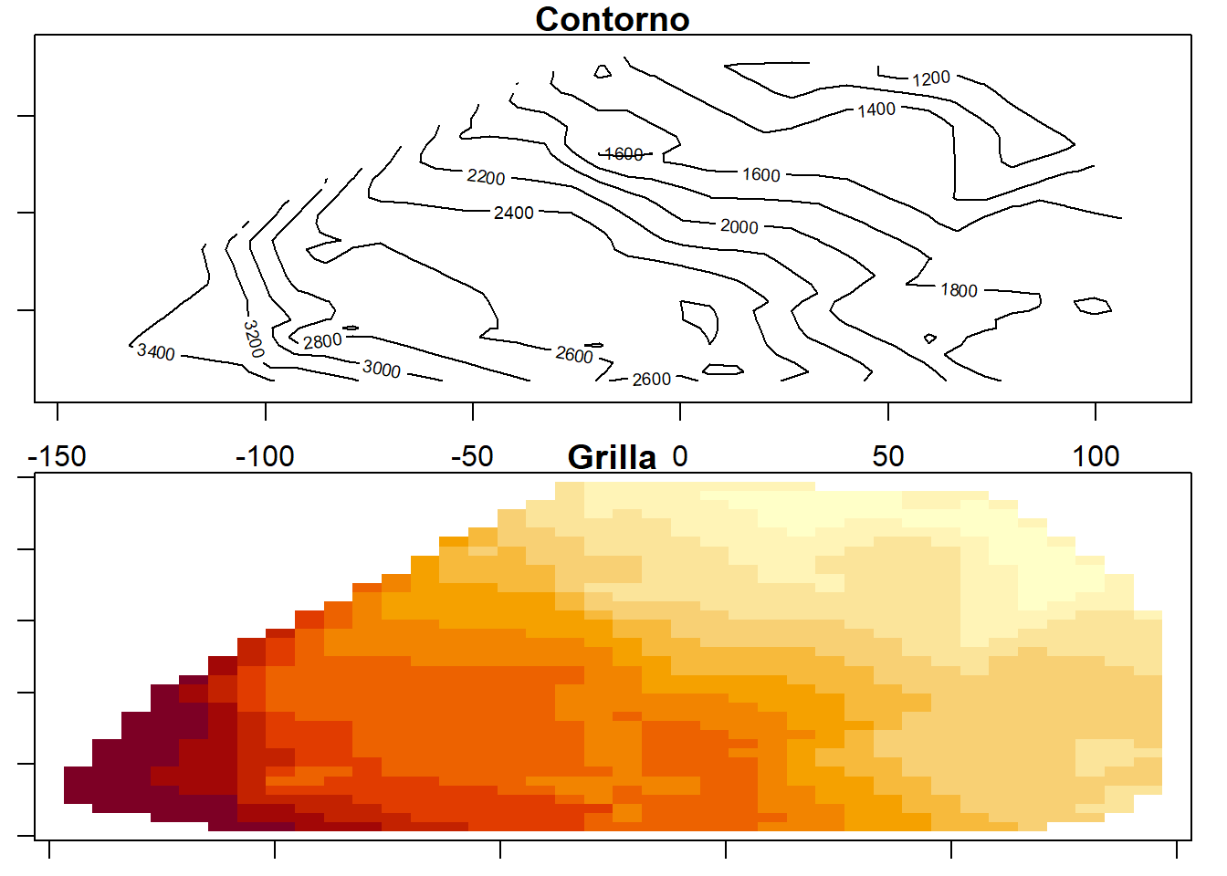
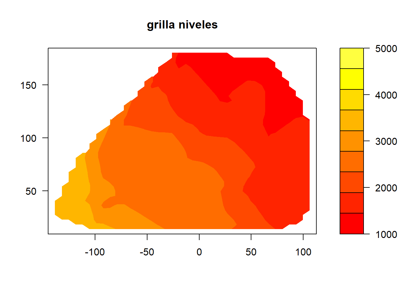
Lectura de datos
aquifer <-read.table("data/aquifer.txt", head =TRUE, dec =",")
      Este             Norte          Profundidad
 Min.   :-145.24   Min.   :  9.414   Min.   :1024
 1st Qu.: -21.30   1st Qu.: 33.682   1st Qu.:1548
 Median :  11.66   Median : 59.158   Median :1797
 Mean   :  16.89   Mean   : 79.361   Mean   :2002
 3rd Qu.:  70.90   3rd Qu.:131.825   3rd Qu.:2540
 Max.   : 112.80   Max.   :184.766   Max.   :3571
Number of data points: 85

Coordinates summary
         Este     Norte
min -145.2365   9.41441
max  112.8045 184.76636

Distance summary
        min         max
  0.2211656 271.0615463

Data summary
    Min.  1st Qu.   Median     Mean  3rd Qu.     Max.
1024.000 1548.000 1797.000 2002.282 2540.000 3571.000
kappa not used for the wave correlation function
---------------------------------------------------------------
likfit: likelihood maximisation using the function optim.
likfit: Use control() to pass additional
         arguments for the maximisation function.
        For further details see documentation for optim.
likfit: It is highly advisable to run this function several
        times with different initial values for the parameters.
likfit: WARNING: This step can be time demanding!
---------------------------------------------------------------
likfit: end of numerical maximisation.
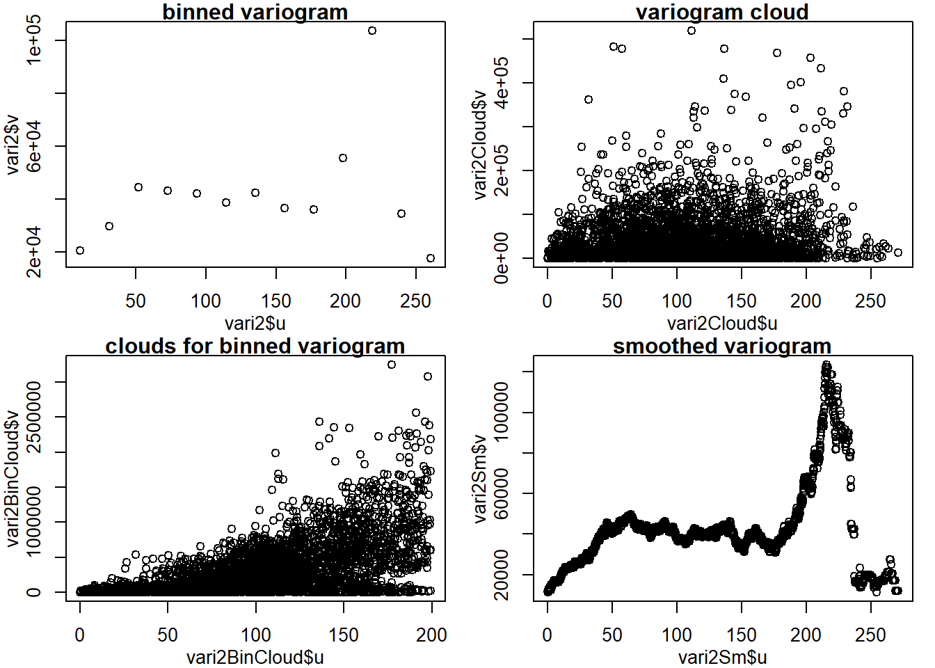
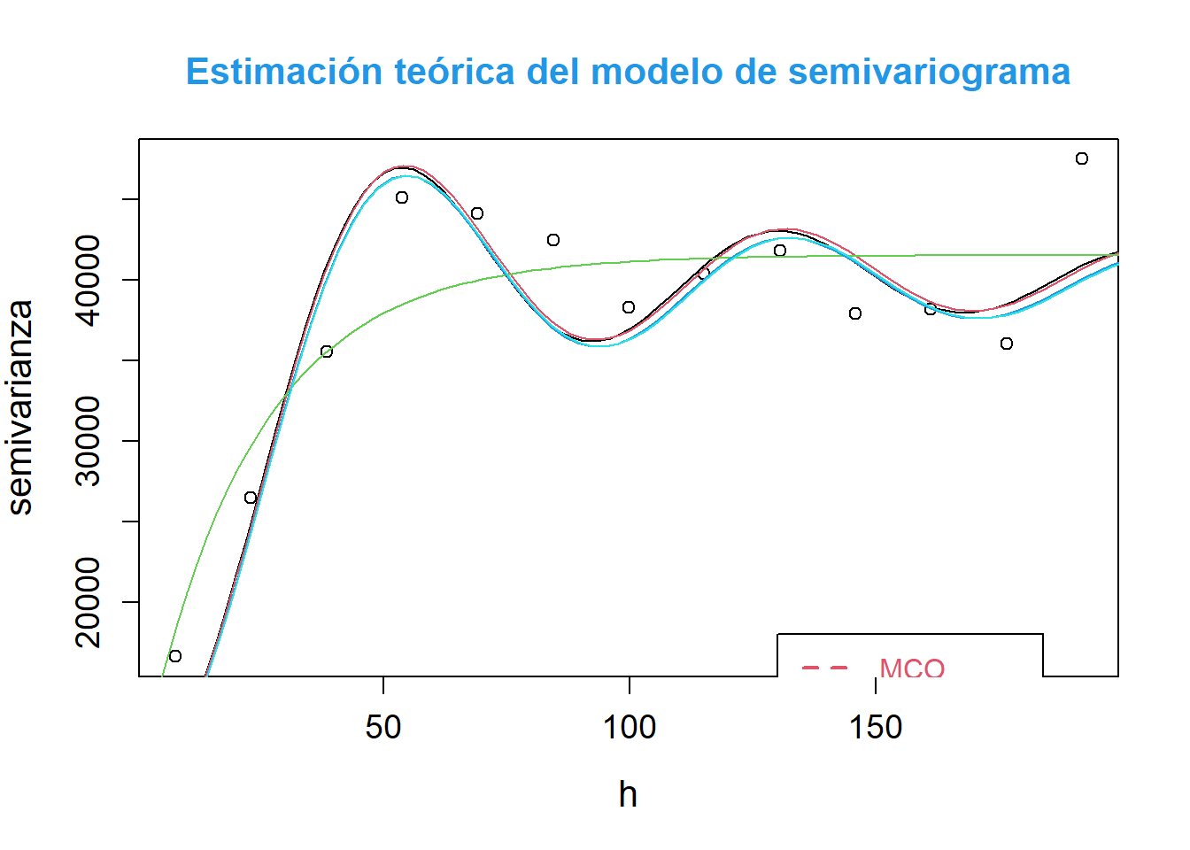
plot(var1$u,var1$v,xlab ="h",ylab ="semivarianza",cex.lab =1.3,cex.axis =1.2,main ="Estimación teórica del modelo de semivariograma",col.main =4, cex.main =1.3)lines(fitvar1, col =1)lines(fitvar2, col =2)lines(fitvar3, col =3)lines(fitvar4, col =4)lines(fitvar5, col =5)legend(130, 18000,c("MCO", "MCPnpairs", "MCPcressie", "ML", "REML"),lwd =2,lty =2:7,col =2:7,box.col =9,text.col =2:7)
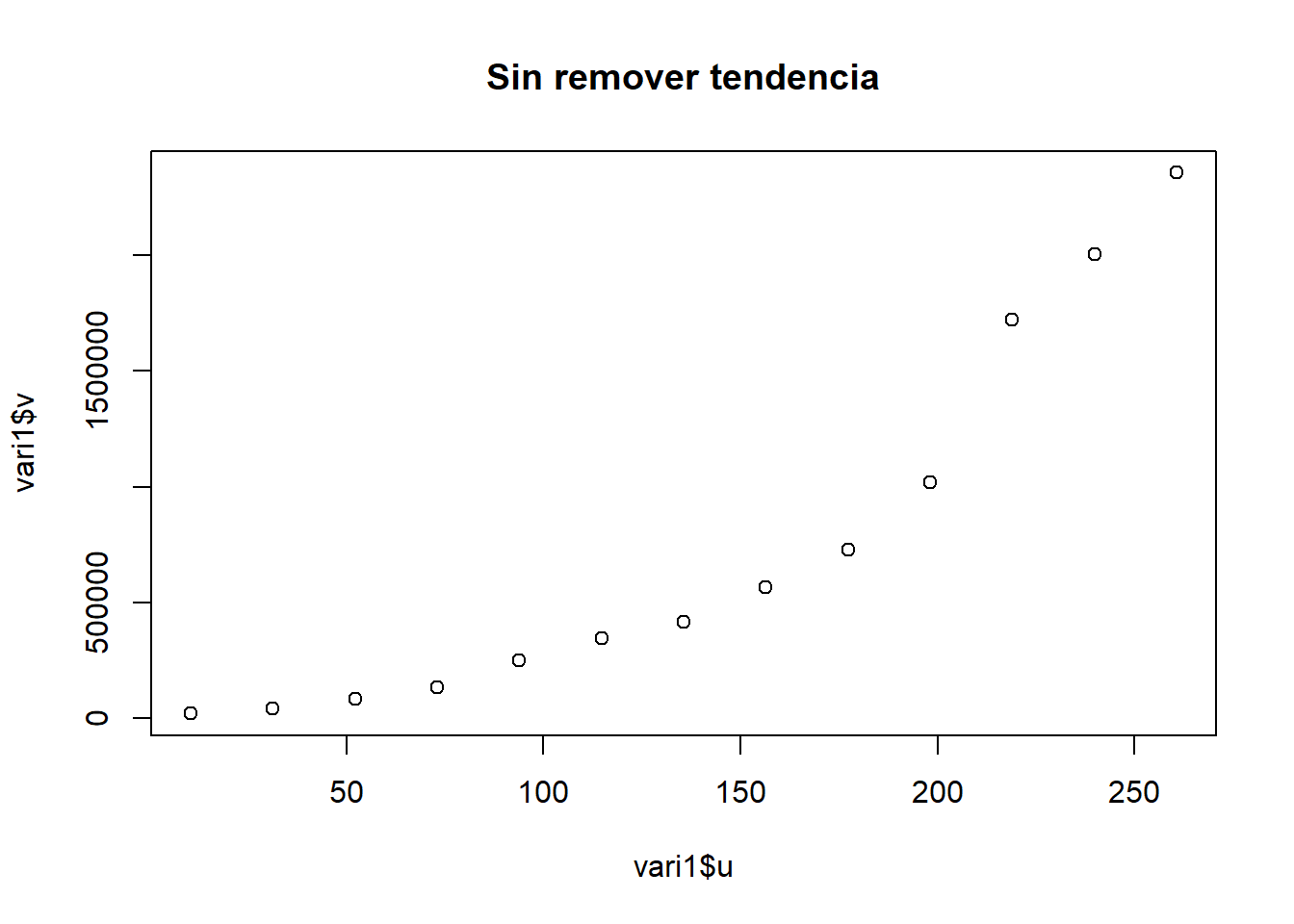
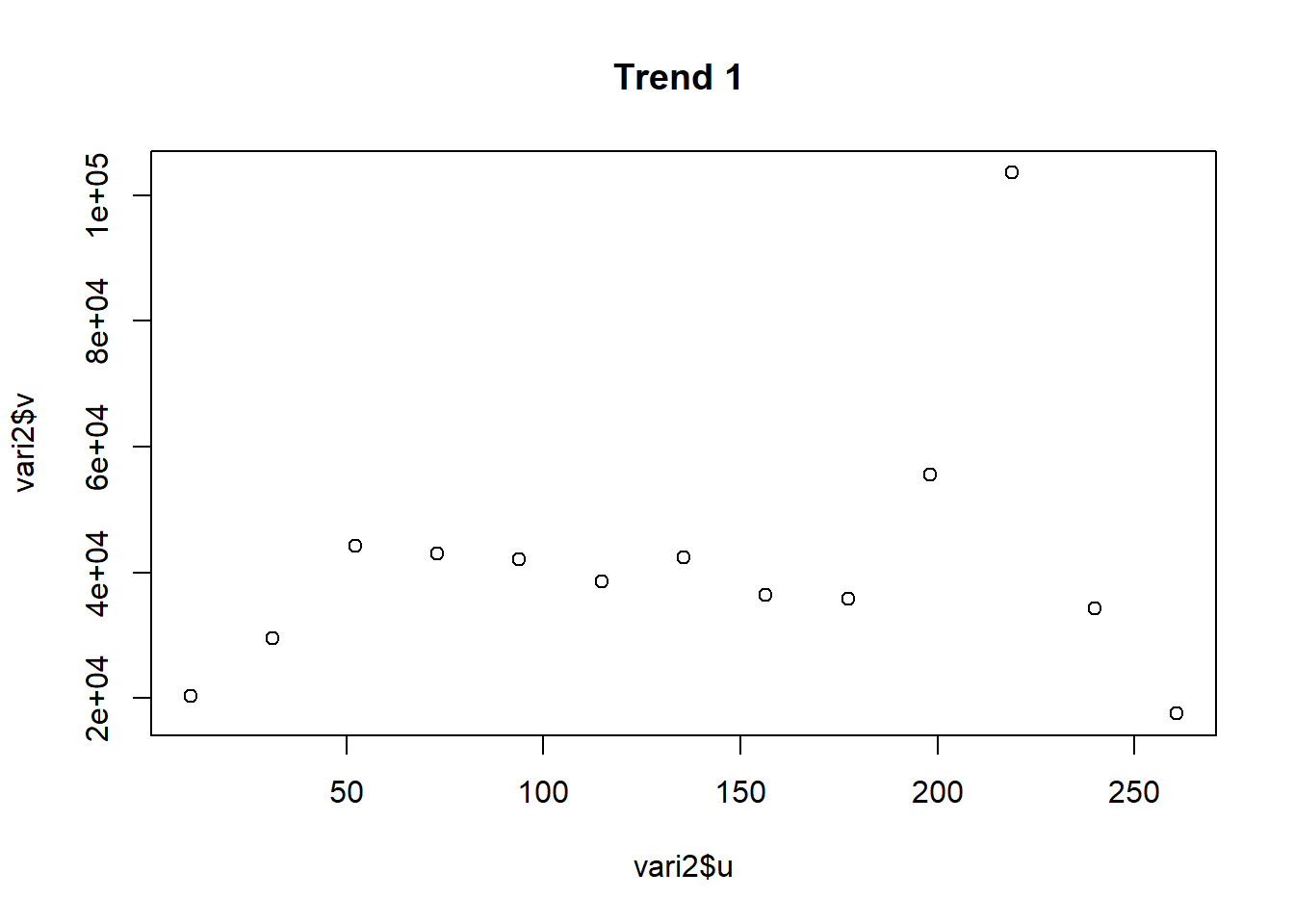
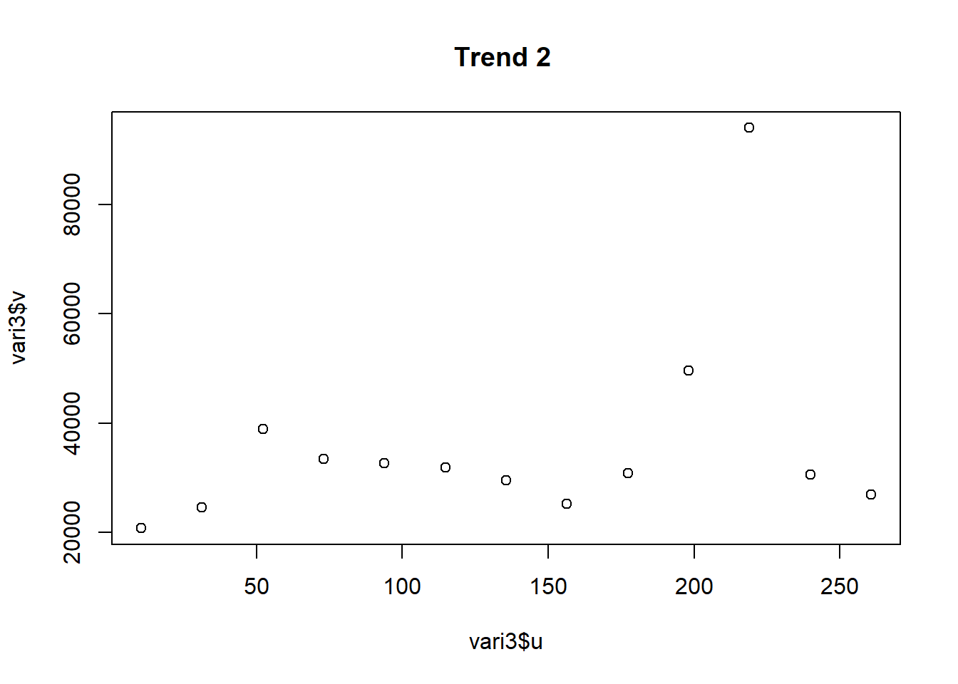
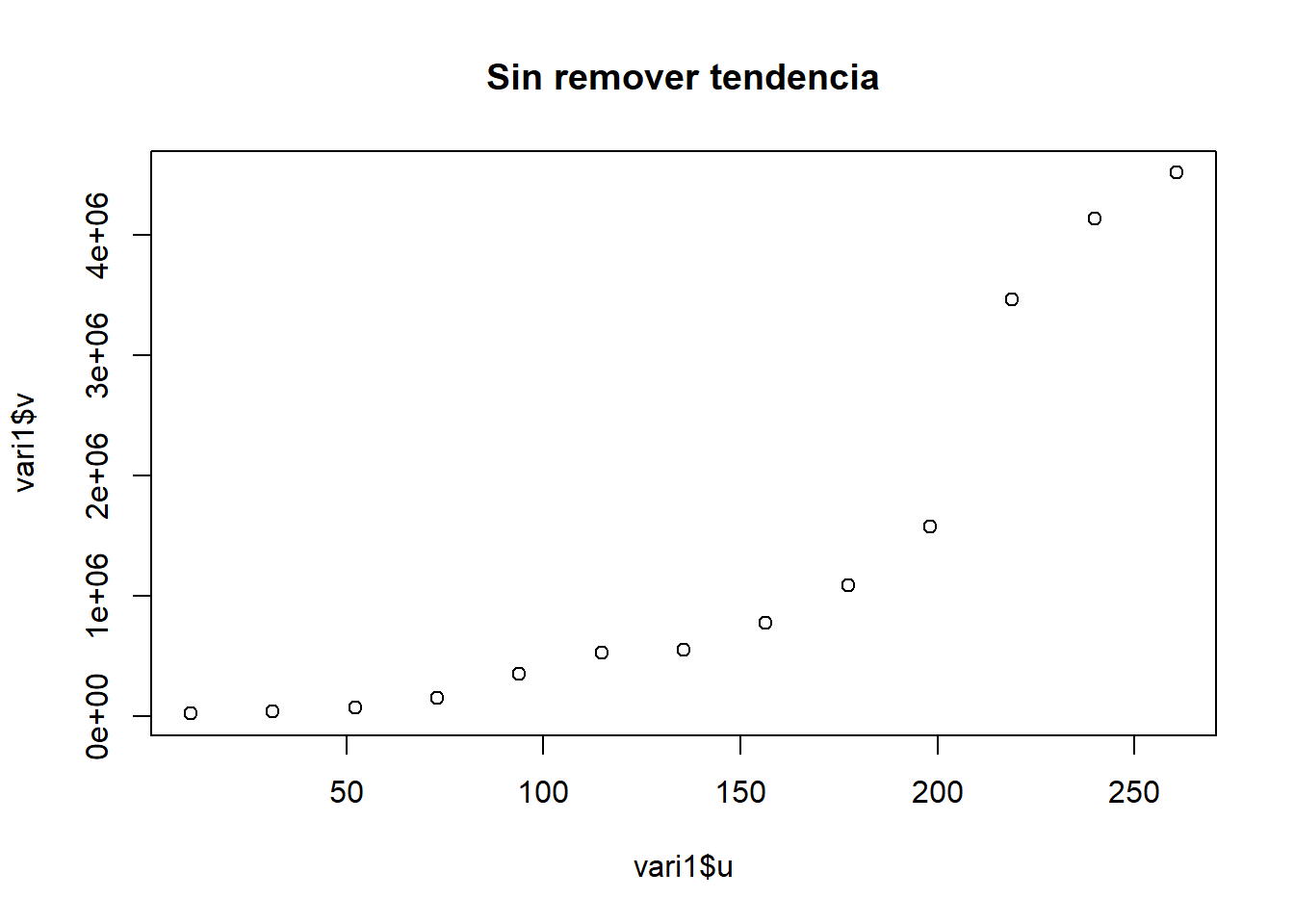
Esta es una alternativa al modelamiento de la media cuando los modelos de regresión polinómicos usuales no logran el objetivo de eliminar la tendencia ya sea porque el tipo de tendencia corresponde mas a unas ventanas móviles o porque hay presentes datos atípicos.
n_x <-4n_y <-6x <-seq(0, 1, len = n_x)y <-seq(0, 1, len = n_y)coordenadas <-as.data.frame(expand.grid(x, y))names(coordenadas) <-c("X", "Y")
Encabezado coordenadas
X
Y
0.0000000
0.0
0.3333333
0.0
0.6666667
0.0
1.0000000
0.0
0.0000000
0.2
0.3333333
0.2
Definición de objeto VGM
Esto define un objeto vgm que es el tipo de objeto que usa el paquete gstat para los modelos teóricos de variograma. Con este objeto se pueden definir modelos anidados.